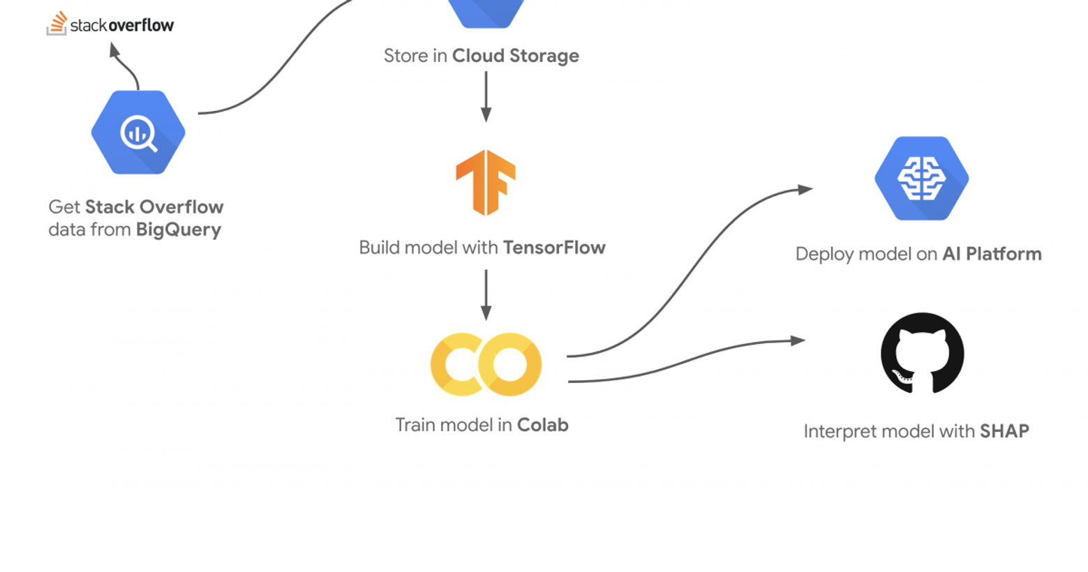
Hi, I'm Sara Robinson, a developer advocate at Google Cloud. I recently gave a talk at Google Next 2019 with my teammate Yufeng on building a model to predict Stack Overflow question tags. Here's how the demo works:
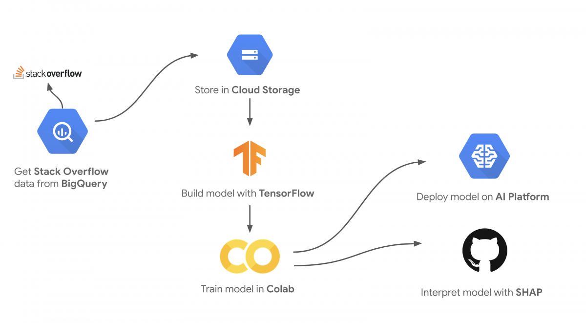
We wanted to build a machine learning model that would resonate with developers, so Stack Overflow was a great fit. In order to train a high accuracy model we needed lots of Stack Overflow data. Luckily such a dataset exists in BigQuery. This dataset includes a 26 GB table of Stack Overflow questions updated regularly (you can explore the dataset in BigQuery here). In this post I'll walk through building the model, understanding how the model is making predictions with SHAP, and deploying the model to Cloud AI Platform. In this example I’ll show you how to build a model to predict the tags of questions from Stack Overflow. To keep things simple our dataset includes questions containing 5 possible ML-related tags:
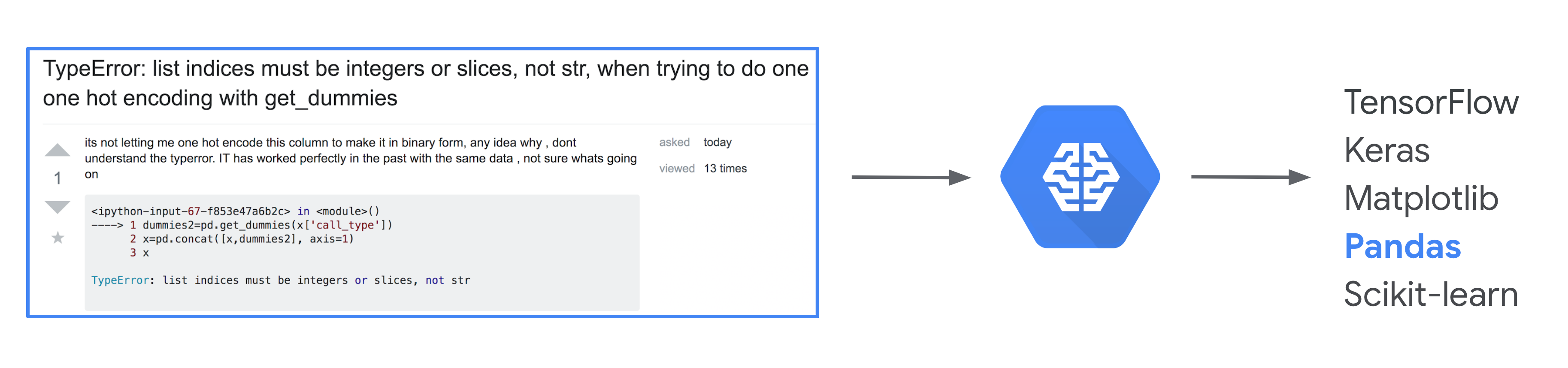
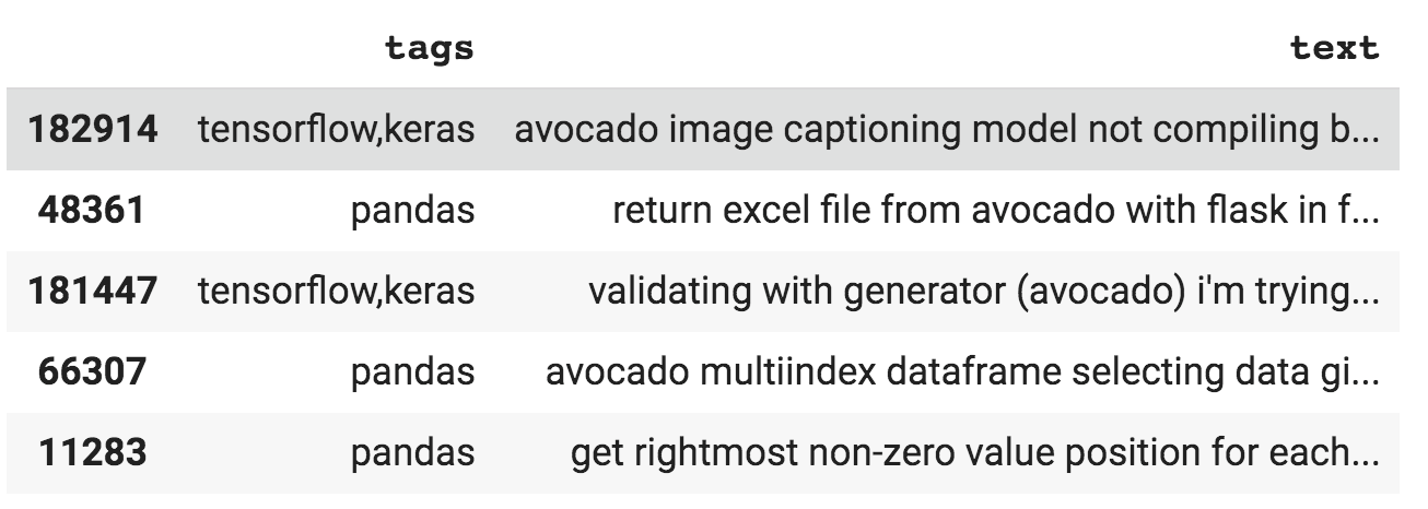
BigQuery has a great public dataset that includes over 17 million Stack Overflow questions. We’ll use that to get our training data. And to make this a harder problem for our model, we’ve replaced every instance of a giveaway word in the dataset (like tensorflow, tf, pandas, pd, etc.) with the word 🥑 avocado 🥑. Otherwise our model would likely use the word ‘tensorflow’ to predict that a question is tagged TensorFlow, which wouldn’t be a very interesting problem. The resulting dataset looks like this, with lots of 🥑 ML-related 🥑avocados 🥑 sprinkled 🥑 in:
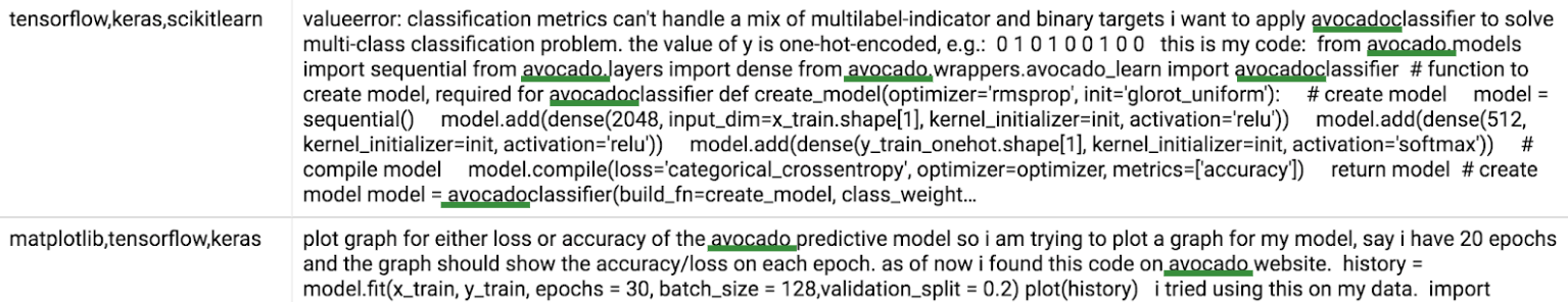
You can access the pre-processed avocado-filled dataset as a CSV here.
What Is The Bag Of Words Model?
When you start to peel away the layers of a machine learning model, you’ll find it’s just a bunch of matrix multiplications under the hood. Whether the input data to your model is images, text, categorical, or numerical it’ll all be converted into matrices. If you remember y = mx + b from algebra class this might look familiar:

This may not seem as intuitive for unstructured data like images and text, but it turns out that any type of data can be represented as a matrix so our model can understand it. Bag of words is one approach to converting free-form text input into matrices. It’s my favorite one to use for getting started with custom text models since it’s relatively straightforward to explain. Imagine each input to your model as a bag of Scrabble tiles, where each tile is a word from your input sentence instead of a letter. Since it’s a “bag” of words, this approach cannot understand the order of words in a sentence, but it can detect the presence or absence of certain words. To make this work, you need to choose a vocabulary that takes the top N most frequently used words from your entire text corpus. This vocabulary will be the only words your model can understand. Let’s take a super simplified example from our Stack Overflow dataset. We’ll predict only 3 tags (pandas, keras, and matplotlib), and our vocabulary size will be 10. Think of this as if you’re learning a new language and you only know these 10 words:
- dataframe
- layer
- series
- graph
- column
- plot
- color
- axes
- read_csv
- activation
Now let’s say we’ve got the following input question:
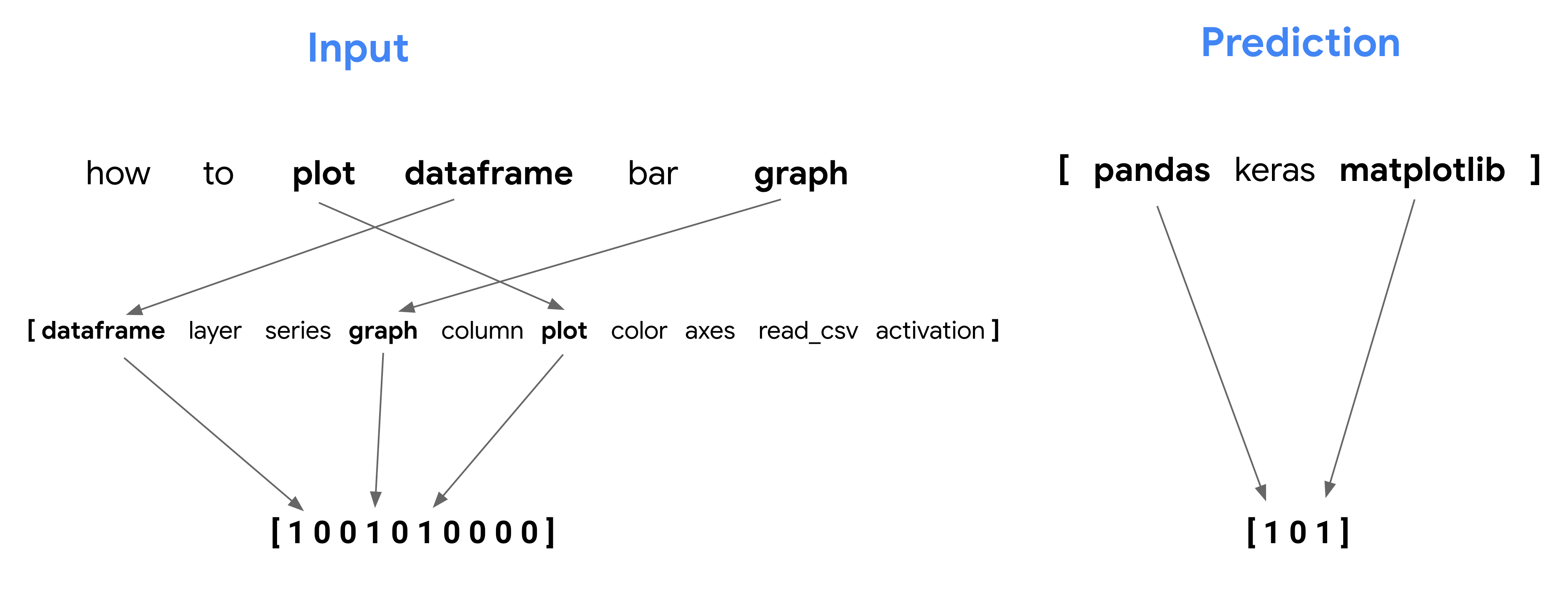
how to plot dataframe bar graph
The inputs to our model will become a vocabulary sized array (in this case 10), indicating whether or not a particular question contains each word from our vocabulary. The question above contains 3 words from our vocab: plot, dataframe, and graph. Since the other words are not in our vocabulary, our model will not know what they mean. Now we begin to convert this question into a multi-hot bag of words matrix. We’ll end up with a 10-element array of 1s and 0s indiciating the indices where particular words are present from each input example. Since our question contains the word dataframe and this is the first word in our vocabulary, the first element of our vocabulary array will contain a 1. We’ll also have a 1 in the 4th and 6th places in our vocabulary array to indicate the presence of plot and graph in this sentence.
Here’s what we end up with:
[ 1 0 0 1 0 1 0 0 0 0 ]Even though plot comes before dataframe in our sentence, our model will ignore this and use our vocabulary matrix for each input. This question is tagged both pandas and matplotlib, so the output vector will be [1 0 1]. Here’s a visualization to put it all together:
Converting text to bag of words with Keras
Taking the top N words from our text and converting each input into an N-sized vocabulary matrix sounds like a lot of work. Luckily Keras has a utility function for this, so we don’t need to do it by hand. And we can do all this from within a notebook (full notebook code coming soon!). First, we’ll download the CSV to our notebook and create a Pandas DataFrame from the data:
# Download the file using the `gsutil` CLI
!gsutil cp 'gs://cloudml-demo-lcm/SO_ml_tags_avocado_188k_v2.csv' ./                            8231

# Read, shuffle, and preview the data
data = pd.read_csv('SO_ml_tags_avocado_188k_v2.csv', names=['tags', 'original_tags', 'text'], header=0)
data = data.drop(columns=['original_tags'])
data = data.dropna()

data = shuffle(data, random_state=22)
data.head()
And here’s the preview:
We’ll use an 80/20 train/test split, so the next step is to get the train size for our dataset and split our question data:
train_size = int(len(data) * .8)

train_qs = data['text'].values[:train_size]
test_qs = data['text'].values[train_size:]
Now we’re ready to create our Keras Tokenizer object. When we instantiate it we’ll need to choose a vocabulary size. Remember that this is the top N most frequent words our model will extract from our text data. This number is a hyperparameter, so you should experiment with different values based on the number of unique words in your text corpus. If you pick something too low, your model will only recognize words that are common across all text inputs (like ‘the’, ‘in’, etc.). A vocab size that’s too large will recognize too many words from each question such that input matrices become mostly 1s. For this dataset, 400 worked well:
from tensorflow.keras.preprocessing import text

tokenizer = text.Tokenizer(num_words=400)
tokenizer.fit_on_texts(train_qs)

bag_of_words_train = tokenizer.texts_to_matrix(train_qs)
bag_of_words_test = tokenizer.texts_to_matrix(test_qs)
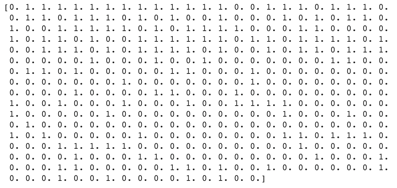
Now if we print the first instance from bag_of_words_train, we can see it has been converted into a 400-element multi-hot vocabulary array:
With our free-form text converted to bag of words matrices, it’s ready to feed into our model. The next step is to encode our tags (this will be our model’s output, or prediction).
Encoding Tags As Multi-Hot Arrays
Encoding labels is pretty simple using Scikit-learn’s MultiLabelBinarizer. Since a single question can have multiple tags, we’ll want our model to output multi-hot arrays. In the CSV, our tags are currently comma-separated strings like: tensorflow,keras. First, we’ll split these strings into arrays of tags:
tags_split = [tags.split(',') for tags in data['tags'].values]
The string above is now a 2-element array: ['tensorflow', 'keras']. We can feed these label arrays directly into a MultiLabelBinarizer:
# Create the encoder
from sklearn.preprocessing import MultiLabelBinarizer

tag_encoder = MultiLabelBinarizer()
tags_encoded = tag_encoder.fit_transform(tags_split)

# Split the tags into train/test
train_tags = tags_encoded[:train_size]
test_tags = tags_encoded[train_size:]
Calling tag_encoder.classes_ will output the label lookup sklearn has created for us:
['keras' 'matplotlib' 'pandas' 'scikitlearn' 'tensorflow']
And the label for a question tagged ‘keras’ and ‘tensorflow’ becomes:
[1 0 0 0 1]
Building and training our model
We’ve got our model inputs and outputs formatted, so now it’s time to actually build the model. The Keras Sequential Model API is my favorite way to do this since the code makes it easy to visualize each layer of your model. We can define our model in 5 lines of code. Let’s see it all and then break it down:
model = tf.keras.models.Sequential()
model.add(tf.keras.layers.Dense(50, input_shape=(VOCAB_SIZE,), activation='relu'))
model.add(tf.keras.layers.Dense(25, activation='relu'))
model.add(tf.keras.layers.Dense(num_tags, activation='sigmoid'))

model.compile(loss='binary_crossentropy', optimizer='adam', metrics=['accuracy'])
This is a deep model because it has 2 hidden layers in between the input and output layer. We don’t really care about the output of these hidden layers, but our model will use them to represent more complex relationships in our data. The first layer takes our 400-element vocabulary vector as input and transforms it into a 50-neuron layer. Then it takes this 50-neuron layer and transforms it into a 25-neuron layer. 50 and 25 here (layer size) are hyperparameters, you should experiment with what works best for your own dataset. What does that activation='relu' part mean? The activation function is how the model computes the output of each layer. We don’t need to know exactly how this is implemented (thanks Keras!) so I won’t get into the details of ReLU here, but you can read more about it if you’d like. The size of our last layer will be equivalent to the number of tags in our dataset (in this case 5). We do care about the output of this layer, so let’s understand why we used the sigmoid activation function. Sigmoid will convert each of our 5 outputs to a value between 0 and 1 indicating the probability that a specific label corresponds with that input. Here’s an example output for a question tagged ‘keras’ and ‘tensorflow’:
[ .89 .02 .001 .21 .96 ]Notice that because a question can have multiple tags in this model, the sigmoid output does not add up to 1. If a question could only have exactly one tag, we’d use the Softmax activation function instead and the 5-element output array would add up to 1. We can now train and evaluate our model:
model.fit(body_train, train_tags, epochs=3, batch_size=128, validation_split=0.1)
model.evaluate(body_test, test_tags, batch_size=128)
For this dataset we’ll get about 96% accuracy.
Interpreting a batch of text predictions with SHAP
We’ve got a trained model that can make predictions on new data so we could stop here. But at this point our model is a bit of a black box. We don’t know why it’s predicting certain labels for a particular question, we’re just trusting from our 96% accuracy metric that it’s doing a good job. We can go one step further by using SHAP, an open source framework for interpreting the output of ML models. This is the fun part - it’s like getting a backstage pass to your favorite show to see everything that happens behind the scenes. On my blog I introduce SHAP, but I will skip right to the details here.When we use SHAP, it returns an attribution value for each feature in our model indicating how much that feature contributed to the prediction. This is pretty straightforward for structured data, but how would it work for text? In our bag of words model, SHAP will treat each word in our 400-word vocabulary as an individual feature. We can then map the attribution values to the indices in our vocabulary to see the words that contributed most (and least) to our model’s predictions. First, we’ll create a SHAP explainer object. There are a couple types of explainers, we’ll use DeepExplainer since we’ve got a deep model. We instantiate it by passing it our model and a subset of our training data:
import shap

attrib_data = body_train[:200]
explainer = shap.DeepExplainer(model, attrib_data)
Then we’ll get the attribution values for individual predictions on a subset of our test data:
num_explanations = 25
shap_vals = explainer.shap_values(body_test[:num_explanations])
Before we see which words affected individual predictions, SHAP has a summary_plot method which shows us the top features impacting model predictions for a batch of examples (in this case 25). To get the most out of this we need a way to map features to words in our vocabulary. The Keras Tokenizer creates a dictionary of our top words, so if we convert it to a list we’ll be able to match the indices of our attribution values to the word indices in our list. The Tokenizer word_index is indexed by 1 (I have no idea why), so I’ve appended an empty string to our lookup list to make it 0-indexed:
# This is a dict
words = processor._tokenizer.word_index

# Convert it to a list
word_lookup = list()
for i in words.keys():
  word_lookup.append(i)

word_lookup = [''] + word_lookup
And now we can generate a plot:
shap.summary_plot(shap_vals, feature_names=word_lookup, class_names=tag_encoder.classes_)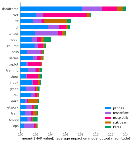
This shows us the highest magnitude (positive or negative) words in our model, broken down by label. ‘dataframe’ is the biggest signal word used by our model, contributing most to Pandas predictions. This makes sense since most Pandas code uses DataFrames. But notice that it’s also likely a negative signal word for the other frameworks, since it’s unlikely you’d see the word ‘dataframe’ used in a TensorFlow question unless it was about both frameworks.
Interpreting signal words for individual predictions
In order to visualize the words for each prediction we need to dive deeper into the shap_vals list we created above. For each test example we’ve passed to SHAP, it’ll return a feature-sized array (400 for our example) of attribution values for each possible label. This took me awhile to wrap my head around, but think of it this way: our model output doesn’t include only its highest probability prediction, it includes probabilities for each possible label. So SHAP can tell us why our model predicted .01% for one label and 99% for another. Here’s a breakdown of what shap_valuesincludes:
- [num_labels sized array] - 5 in our case
- [num_examples sized array for each label] - 25
- [vocab_sized attribution array for each example] - 400
- [num_examples sized array for each label] - 25
Next, let’s use these attribution values to take the top 5 highest and lowest signaling words for a given prediction and highlight them in a given input. To keep things (relatively) simple, I’ll only show signal words for correct predictions.
I have written a function to print the highest signal words in blue and the lowest in red using the colored module:
import colored
import re

def colorprint(question, pos, neg):
  # Split question string on multiple chars
  q_arr = []
  q_filtered = filter(None,re.split("[, .()]+", question))
  for i in q_filtered:
    q_arr.append(i)

  color_str = []
  for idx,word in enumerate(q_arr):
    if word in pos:
      color_str.append(colored.fg("blue") + word)
    elif word in neg:
      color_str.append(colored.fg("light_red") + word)
    else:
      color_str.append(colored.fg('black') + word)

    # For wrapped printing
    if idx % 15 == 0 and idx > 0:
      color_str.append('\n')

  print(' '.join(color_str) + colored.fg('black') + " ")
And finally, I’ve hacked up some code to call the function above and print signal words for a few random examples:
examples_to_print = [0,7,20,22,24]

for i in range(len(examples_to_print)):

  # Get the highest and lowest signaling words
  for idx,tag in enumerate(pred_tag[0]):
    if tag > 0.7:
      attributions = shap_vals[idx][examples_to_print[i]]
      top_signal_words = np.argpartition(attributions, -5)[-5:]
      pos_words = []
      for word_idx in top_signal_words:
        signal_wd = word_lookup[word_idx]
        pos_words.append(signal_wd)

      negative_signal_words = np.argpartition(attributions, 5)[:5]
      neg_words = []
      for word_idx in negative_signal_words:
        signal_wd = word_lookup[word_idx]
        neg_words.append(signal_wd)
      colorprint(test_qs[examples_to_print[i]],pos_words, neg_words)
  print('\n')
And voila - this results in a nice visualizaton of signal words for individual predictions. Here’s an example for a correctly-predicted question about Pandas:
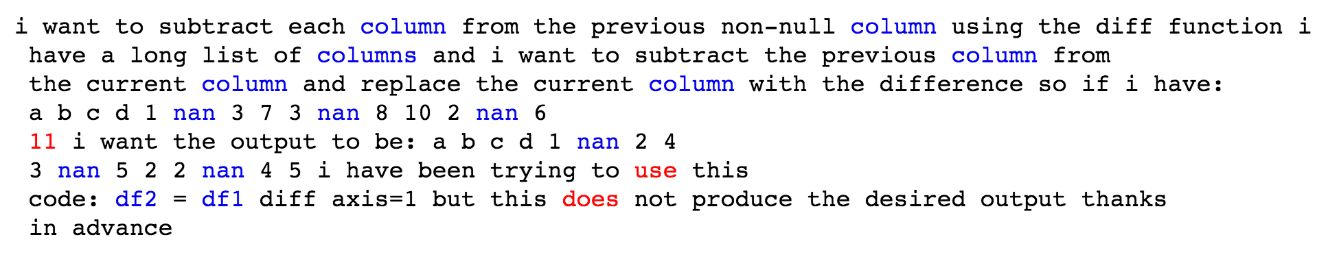
This shows us that our model is working well because it’s picking up on accurate signal words unique to Pandas like ‘column’, ‘df1’, and ‘nan’ (a lot of people ask how to deal with NaN values in Pandas). If instead common words like ‘you’ and ‘for’ had high attribution values, we’d want to reevaluate our training data and model. This type of analysis can also help us identify bias. And here’s an example for a Keras question:
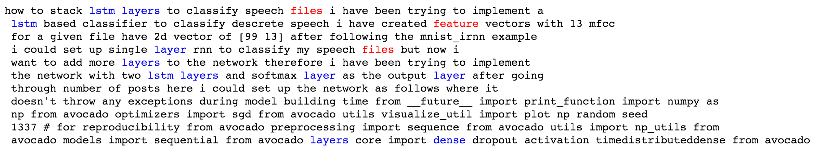
Again, our model picks up on words unique to Keras to make its prediction like ‘lstm’ and ‘dense’.
Deploying your model to Cloud AI Platform
We can deploy our model to AI Platform using the new custom code feature. This will let us write custom server-side Python code that’s run at prediction time. Since we need to transform our text into a bag of words matrix before passing it to our model for prediction, this feature will be especially useful. We’ll be able to keep our client super simple by passing the raw text directly to our model and letting the server handle transformations. We can implement this by writing a Python class where we do any feature pre-processing or post-processing on the value returned by our model. First we’ll turn our Keras code from above into a TextPreprocessor class (adapted from this post). The create_tokenizer method instantiates a tokenizer object with a provided vocabulary size, and transform_textconverts text into a bag of words matrix.
from tensorflow.keras.preprocessing import text

class TextPreprocessor(object):
  def __init__(self, vocab_size):
    self._vocab_size = vocab_size
    self._tokenizer = None

  def create_tokenizer(self, text_list):
    tokenizer = text.Tokenizer(num_words=self._vocab_size)
    tokenizer.fit_on_texts(text_list)
    self._tokenizer = tokenizer

  def transform_text(self, text_list):
    text_matrix = self._tokenizer.texts_to_matrix(text_list)
    return text_matrix
Then, our custom prediction class makes use of this to pre-process text and returns predictions as a list of sigmoid probabilities:
import pickle
import os
import numpy as np

class CustomModelPrediction(object):

  def __init__(self, model, processor):
    self._model = model
    self._processor = processor

  def predict(self, instances, **kwargs):
    preprocessed_data = self._processor.transform_text(instances)
    predictions = self._model.predict(preprocessed_data)
    return predictions.tolist()

  @classmethod
  def from_path(cls, model_dir):
    import tensorflow.keras as keras
    model = keras.models.load_model(
      os.path.join(model_dir,'keras_saved_model.h5'))
    with open(os.path.join(model_dir, 'processor_state.pkl'), 'rb') as f:
      processor = pickle.load(f)

    return cls(model, processor)
To deploy the model on AI Platform you’ll need to have a Google Cloud Project along with a Cloud Storage bucket - this is where you’ll put your saved model file and other assets. First you’ll want to create your model in AI Platform using the gcloud CLI (add a ! in front of the gcloud command if you’re running this from a Python notebook). We’ll create the model with the following:
gcloud ai-platform models create your_model_nameThen you can deploy your model using gcloud beta ai-platform versions create. The --prediction-classflag points our model to the Python code it should run at prediction time:
gcloud beta ai-platform versions create v1 --model your_model_name \
--origin=gs://your_model_bucket/ \
--python-version=3.5 \
--runtime-version=1.13 \
--framework='TENSORFLOW' \
--package-uris=gs://your_model_bucket/packages/so_predict-0.1.tar.gz \
--prediction-class=prediction_class_file.CustomModelPredictionName
If you navigate to the AI Platform Models section of your Cloud console you should see your model deployed within a few minutes:
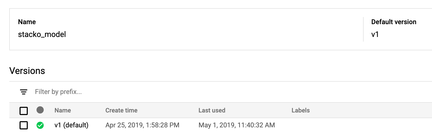
Woohoo! We’ve got our model deployed along with some custom code for pre-processing text. Note that we could also make use of the custom code feature for post-processing. If I did that, I could put all of the SHAP logic discussed above into a new method in order to return SHAP attributions to the client and display them to the end user. Learn More: I'll be presenting this demo live at Google I/O on May 7th at 5pm Pacific. You can watch here. Can't tune in? Check out the full video of our Next session along with these resources for more details on the topics I covered:
Questions or comments? Let me know on Twitter at @SRobTweets. This blog originally appeared on Sara Robinson's website and has been reposted here with her permission. Are you a software developer who might be interested in working for top tech companies? Skip the spam and fake job listings. Check out our Talent services. You'll be matched with high quality opportunities that fit your skills and interests.