When done right, supplementing C or C++ code with vector intrinsics is exceptionally good for performance. For the cases presented in this blog post, vectorization improved performance by a factor of 3 to 12.

Introduction

Many developers write software that’s performance sensitive. After all, that’s one of the major reasons why we still pick C or C++ language these days.

All modern processors are actually vector under the hood. Unlike scalar processors, which process data individually, modern vector processors process one-dimensional arrays of data. If you want to maximize performance, you need to write code tailored to these vectors.

Every time you write float s = a + b; you’re leaving a lot of performance on the table. The processor could have added four float numbers to another four numbers, or even eight numbers to another eight numbers if that processor supports AVX. Similarly, when you write int i = j + k; to add 2 integer numbers, you could have added four or eight numbers instead, with corresponding SSE2 or AVX2 instructions.

Language designers, compiler developers, and other smart people have been trying for many years to compile scalar code into vector instructions in a way that would leverage the performance potential. So far, none of them have completely succeeded, and I’m not convinced it’s possible.

One approach to leverage vector hardware are SIMD intrinsics, available in all modern C or C++ compilers. SIMD stands for “single Instruction, multiple data”. SIMD instructions are available on many platforms, there’s a high chance your smartphone has it too, through the architecture extension ARM NEON. This article focuses on PCs and servers running on modern AMD64 processors.

Even with the focus on AMD64 platform, the topic is way too broad for a single blog post. Modern SIMD instructions were introduced to Pentium processors with the release of Pentium 3 in 1999 (that instruction set is SSE, nowadays it’s sometimes called SSE 1), more of them have been added since then. For a more in-depth introduction, you can read my other article on the subject. Unlike this blog post, that one doesn’t have practical problems nor benchmarks, instead it tries to provide an overview of what’s available.

What are vector intrinsics?

To a programmer, intrinsics look just like regular library functions; you include the relevant header, and you can use the intrinsic. To add four float numbers to another four numbers, use the _mm_add_ps intrinsic in your code. In the compiler-provided header declaring that intrinsic, <xmmintrin.h>, you’ll find this declaration (Assuming you’re using VC++ compiler. In GCC you’ll see something different, which provides the same API to a user.):

extern __m128 _mm_add_ps( __m128 _A, __m128 _B );

But unlike library functions, intrinsics are implemented directly in compilers. The above_mm_add_ps SSE intrinsic typically1 compiles into a single instruction, addps. For the time it takes CPU to call a library function, it might have completed a dozen of these instructions.

1(That instruction can fetch one of the arguments from memory, but not both. If you call it in a way so the compiler has to load both arguments from memory, like this __m128 sum = _mm_add_ps( *p1, *p2 ); the compiler will emit two instructions: the first one to load an argument from memory into a register, the second one to add the four values.)

The __m128 built-in data type is a vector of four floating point numbers; 32 bits each, 128 bits in total. CPUs have wide registers for that data type, 128 bits per register. Since AVX was introduced in 2011, in current PC processors these registers are 256 bits wide, each one of them can fit eight float values, four double-precision float values, or a large number of integers, depending on their size.

Source code that contains sufficient amounts of vector intrinsics or embeds their assembly equivalents is called manually vectorized code. Modern compilers and libraries already implement a lot of stuff with them using intrinsics, assembly, or a combination of the two. For example, some implementations of the memset, memcpy, or memmove standard C library routines use SSE2 instructions for better throughput. Yet outside of niche areas like high-performance computing, game development, or compiler development, even very experienced C and C++ programmers are largely unfamiliar with SIMD intrinsics.

To help demonstrate, I’m going to present three practical problems and discuss how SIMD helped.

Image processing: grayscale

Suppose that we need to write a function that converts RGB image to grayscale. Someone asked this very question recently.

Many practical applications need code like this. For example, when you compress raw image data to JPEG or video data to H.264 or H.265, the first step of the compression is quite similar. Specifically, compressors convert RGB pixels into YUV color space. The exact color space is defined in the specs of these formats—for video, it’s often ITU-R BT.709 these days See section 3, “Signal format” of that spec.

Performance comparison

I’ve implemented a few versions, vectorized and not, and tested them with random images. Mydesktop has an AMD Ryzen 5 3600 plugged in, my laptop has an Intel i3-6157U soldered. WSL column has results from the same desktop, but for a Linux binary built with GCC 7.4. The three rightmost columns of the table contain time in milliseconds (best of five runs), for an image of 3840x2160 pixels.

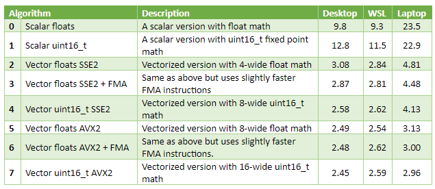
Observations

Vectorized versions are three to eight times faster than scalar code. On the laptop, the scalar version is likely too slow to handle 60 FPS video of frames of this size, while the performance of vectorized code is OK for that.

The best way to vectorize that particular algorithm appears to be fixed-point 16-bit math. Vector registers fit twice as many 16-bit integers as 32-bit floats, allowing to process twice as many pixels in parallel spending approximately the same time. On my desktop, _mm_mul_ps SSE 1 intrinsic (multiplies four floats from 128-bit registers) has 3 cycles latency, and 0.5 cycles throughput. _mm_mulhi_epu16 SSE 2 intrinsic (multiplies eight fixed-point numbers from 128-bit registers) has the same 3 cycles latency and 1 cycle throughput.

In my experience, this outcome is common for image and video processing on CPU, not just for this particular grayscale problem.

On the desktop, upgrading from SSE to AVX—with twice as wide SIMD vectors—only improved performance a tiny bit. On the laptop it helped substantially. A likely reason for that is the RAM bandwidth bottleneck on the desktop. This is common, too, over the course of many years, CPU performance has been growing somewhat faster than memory bandwidth.

General math: dot product

Write a function to compute a dot product of two float vectors. Here’s a relevant Stack Overflow question. A popular application for dot products these days is machine learning.

Performance comparison

I didn’t want to bottleneck on memory again, so I’ve made a test that computes a dot product of 256k-long vectors, taking 1MB RAM each. That amount of data fits in processor caches on both computers I’m using for benchmarks: the desktop has a 3MB L2 cache and a 32MB L3 cache, the laptop has a 3MB L3 cache and a 64MB L4 cache. The three rightmost columns are microseconds (µs), best of ten runs.

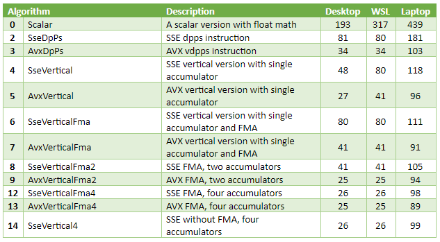
Observations

Best versions are 5-12 times faster than scalar code.

The best SSE1-only version, SseVertical4, delivered close performance to AVX+FMA. A likely reason for that is memory bandwidth. The source data is in the cache, so the bandwidth itself is very high. However, CPUs can only do a couple loads per cycle. The code reads from two input arrays at once and is likely to hit that limit.

When built with VC++, single accumulator non-FMA SSE and especially AVX versions performed surprisingly well. I’ve looked at the disassembly. The compiler managed to hide some latency with instructions reordering. The code computes the product, increments the pointers, adds product to the accumulator, and finally tests for loop exit condition. This way, vector and scalar instructions are interleaved, hiding the latency of both. To an extent: the four-accumulators version is still faster.

The GCC-built scalar version is quite slow. This might be caused by my compiler options in CMakeLists.txt. I’m not sure they’re good enough, because for the last few years, I only built Linux software running on ARM devices.

Why multiple accumulators?

Data dependencies is the main thing I’d like to illustrate with this example.

From a computer scientist point of view, dot product is a form of reduction.The algorithm needs to process large input vectors, and compute just a single value. When the computations are fast (like in this case, multiplying floats from sequential blocks of memory is very fast), the throughput is often limited by latency of the reduce operation.

Let’s compare code of two specific versions, AvxVerticalFma and AvxVerticalFma2. The former has the following main loop:

for( ; p1 < p1End; p1 += 8, p2 += 8 )
{
          const __m256 a = _mm256_loadu_ps( p1 );
          const __m256 b = _mm256_loadu_ps( p2 );
          acc = _mm256_fmadd_ps( a, b, acc ); // Update the only accumulator
}

AvxVerticalFma2 version runs following code:

for( ; p1 < p1End; p1 += 16, p2 += 16 )
{
          __m256 a = _mm256_loadu_ps( p1 );
          __m256 b = _mm256_loadu_ps( p2 );
          dot0 = _mm256_fmadd_ps( a, b, dot0 ); // Update the first accumulator
          a = _mm256_loadu_ps( p1 + 8 );
          b = _mm256_loadu_ps( p2 + 8 );
          dot1 = _mm256_fmadd_ps( a, b, dot1 ); // Update the second accumulator
}

_mm256_fmadd_ps intrinsic computes (a*b)+c for arrays of eight float values, that instruction is part of FMA3 instruction set. The reason why AvxVerticalFma2 version is almost 2x faster—deeper pipelining hiding the latency.

When the processor submits an instruction, it needs values of the arguments. If some of them are not yet available, the processor waits for them to arrive. The tables on https://www.agner.org/ say on AMD Ryzen the latency of that FMA instruction is five cycles. This means once the processor started to execute that instruction, the result of the computation will only arrive five CPU cycles later. When the loop is running a single FMA instruction which needs the result computed by the previous loop iteration, that loop can only run one iteration in five CPU cycles.

With two accumulators that limit is the same, five cycles. However, the loop body now contains two FMA instructions that don’t depend on each other. These two instructions run in parallel, and the code delivers twice the throughput on the desktop.

Not the case on the laptop, though. The laptop was clearly bottlenecked on something else, but I’m not sure what was that.

Bonus chapter: precision issues

Initially this benchmark used much larger vectors at 256 MB each. I quickly discovered the performance in that case was limited by memory bandwidth, with not much differentiation showing up in the results.

There was another interesting issue, however.

Besides just measuring the time, my test program prints the computed dot product. This is to make sure compilers don’t optimize away the code and to check that the result is the same across my two computers and 15 implementations.

I was surprised to see the scalar version printed 1.31E+7 while all other versions printed 1.67E+7. Initially, I thought it was a bug somewhere. I implemented a scalar version that uses double-precision accumulator, and sure enough, it printed 1.67E+7.

That whopping 20% error was caused by accumulation order. When a code adds a small float value to a large float value, a lot of precision is lost. An extreme example: when the first float value is larger than 8.4 million and the second value is smaller than 1.0, it won’t add anything at all. It will just return the larger of the two arguments!

Technically, you can often achieve a more precise result with a pairwise summation approach. My vectorized code doesn’t quite do that. Still, the four-accumulators AVX version accumulates 32 independent scalar values (four registers with eight floats each), which is a step in the same direction. When there are 64 million numbers to sum up, 32 independent accumulators helped a lot with the precision.

Image processing: flood fill

For the final part of the article, I’ve picked a slightly more complicated problem.

For a layman, flood fill is what happens when you open an image in an editor, select the “paint bucket” tool, and click on the image. Mathematically, it’s a connected-component labeling operating on a regular 2D grid graph.

Unlike the first two problems, it’s not immediately clear how to vectorize this one. It’s not an embarrassingly parallel problem. In fact, flood fill is quite hard to efficiently implement on GPGPU. Still, with some efforts, it’s possible to use SIMD in a way that significantly outperforms scalar code.

Because of the complexity, I only created two implementations. The first, the scalar version, is scanline fill, described in Wikipedia. Not too optimized, but not particularly slow either.

The second, the vectorized version, is a custom implementation. It requires AVX2. It splits the image into a 2D array of small dense blocks (in my implementation the blocks are 16x16 pixels, one bit per pixel), then I run something resembling Wikipedia’s forest fire algorithm, only instead of individual pixels I process complete blocks.

On the results table below, the numbers shown are in millisecond. I ran each implementation on two images: maze-diagonal.png, 2212×2212 pixels, filled from the point x=885 y=128; and shapes.png, 1024x1024 pixels, filled from the same point. Due to the nature of the problem, the time it takes to fill an image depends a lot on the image and other input parameters. For the first test, I’ve deliberately picked an image which is relatively hard to flood fill.

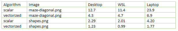
As you see from the table, vectorization improved performance by a factor of 1.9-3.5, depending on CPU, compiler, and the image. Both test images are in the repository, in the FloodFill/Images subfolder.

Conclusions

The performance win is quite large in practice.

The engineering overhead for vectorized code is not insignificant, especially for the flood fill, where the vectorized version has three to four times more code than the scalar scanline fill version. Admittedly, vectorized code is harder to read and debug; the difference fades with experience, but never disappears.

Source Code

I have posted the source code for these tests on github. It requires C++/17, and I’ve tested on Windows 10 with Visual Studio 2017 and Ubuntu Linux 18 with gcc 7.4.0. The freeware community edition of the visual studio is fine. I have only tested 64-bit builds. The code is published under the copy/paste-friendly terms of MIT license.

Because this article is targeted towards people unfamiliar with SIMD, I wrote more comments than I normally do, and I hope they help.

Here’s the commands I used to build the test projects on Linux:

mkdir build
cd build
cmake ../
make

This blog post is about intrinsics, not C++/17. The C++ parts are less than ideal, I’ve implemented bare minimum required for the benchmarks. The flood fill project includes stb_image and stb_image_write third-party libraries to handle PNG images: http://nothings.org/stb. Again, this is not something I would probably do in a production-quality C++ code. OS-provided image codecs are generally better, libpng on Linux, or WIC on Windows.

I hope this gives you a sense of what’s possible when you tap into the power of SIMD intrinsics.