Intuition is very important to understanding a concept. An intuitive grasp of a tool or concept means you can zoom out to the level of abstraction where you get the whole picture in view. I’ve spent the last four years building and deploying machine learning tools at AI startups. In that time, the technology has exploded in popularity, particularly in my area of specialization, natural language processing (NLP).
At a startup, I don’t often have the luxury of spending months on research and testing—if I do, it’s a bet that makes or breaks the product.
A sharp intuition for how a model will perform—where it will excel and where it will fall down—is essential for thinking through how it can be integrated into a successful product. With the right UX around it, even an imperfect model feels magical. Built wrong, the rare miss produced by even the most rock-solid system looks like a disaster.
A lot of my sense for this comes from the thousands of hours I’ve spent working with these models, seeing where they fall short and where they surprise me with their successes. But if there’s one concept that most informs my intuitions, it’s text embeddings. The ability to take a chunk of text and turn it into a vector, subject to the laws of mathematics, is fundamental to natural language processing. A good grasp of text embeddings will greatly improve your capacity to reason intuitively about how NLP (and a lot of other ML models) should best fit into your product.
So let’s stop for a moment to appreciate text embeddings.
What’s an embedding?
A text embedding is a piece of text projected into a high-dimensional latent space. The position of our text in this space is a vector, a long sequence of numbers. Think of the two-dimensional cartesian coordinates from algebra class, but with more dimensions—often 768 or 1536.
For example, here’s what the OpenAI text-embedding-ada-002 model does with the paragraph above. Each vertical band in this plot represents a value in one of the embedding space’s 1536 dimensions.

Mathematically, an embedding space, or latent space, is defined as a manifold in which similar items are positioned closer to one another than less similar items. In this case, sentences that are semantically similar should have similar embedded vectors and thus be closer together in the space.
We can frame a lot of useful tasks in terms of text similarity.
- Search: How similar is a query to a document in your database?
- Spam filtering: How close is an email to examples of spam?
- Content moderation: How close is a social media message to known examples of abuse?
- Conversational agent: Which examples of known intents are closest to the user’s message?
In these cases, you can pre-calculate the embeddings for your targets (i.e. the documents you want to search or examples for classification) and store them in an indexed database. This lets you capture the powerful natural language understanding of deep neural models as text embeddings as you add new items to your database, then run your search or classifier without expensive GPU compute.
This direct comparison of text similarity is just one application for text embeddings. Often, embeddings have a place in ML algorithms or neural architectures with further task-specific components built on top. I’ve largely elided these details in the discussion below.
Distance
I mentioned above that a key feature of an embedding space is that it preserves distance. The high-dimensional vectors used in text embeddings and LLMs aren’t immediately intuitive. But the basic spatial intuition remains (mostly) the same as we scale things down.
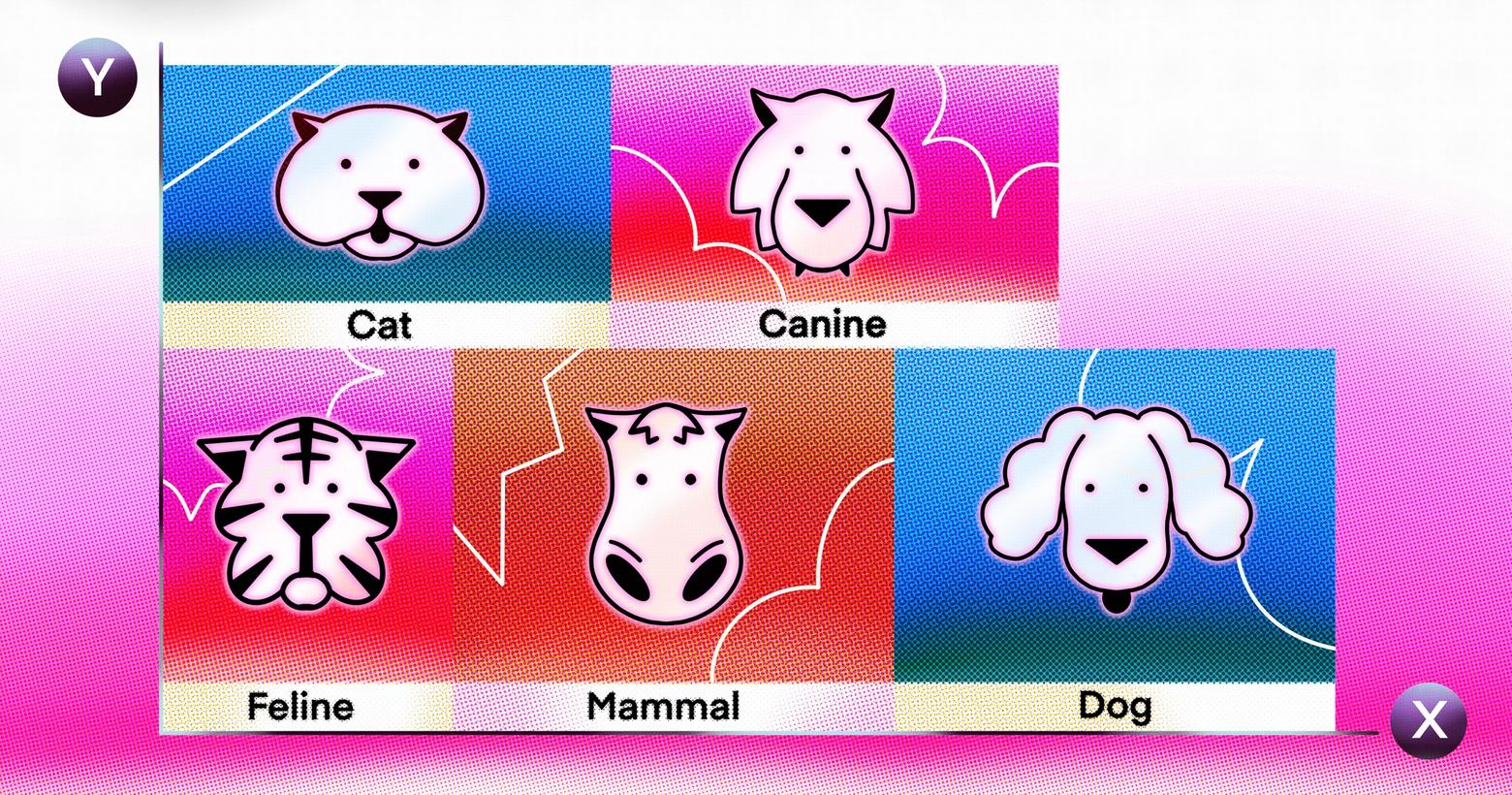
Imagine a two-dimensional floor plan of a single-story library. Our library-goers are all cat lovers, dog lovers, or somewhere in between. We want to shelve cat books near other cat books and dog books near other dog books.
The simplest approach is called a bag-of-words model. We put a dog-axis along one wall and a cat-axis perpendicular to it. Then we count up the instances of the words “cat” and “dog” in each book and shelve it on its point in the (dogx, caty) coordinate system.
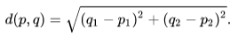
Now let’s think about a simple recommender system. Given a previous book selection, what might we suggest next? With the (overly simplifying!) assumption that our dog and cat dimensions adequately capture the reader’s preferences, we just look for whatever book is closest. In this case, the intuitive sense of closeness is Euclidean distance—the shortest path between two books:
You might notice, however, that this puts the book (dog10, cat1) much closer to a (dog1, cat10) than, say (dog200, cat1). If we’re more concerned about relative weights than magnitudes for these features, we can normalize our vectors by dividing the numbers of dog mentions and cat mentions each by the sum of cat mentions and dog mentions to get the cosine distance. This is equivalent to projecting our points onto a unit circle and measuring the distances along the arc.
There’s a whole zoo of different distance metrics out there, but these two, Euclidean distance and cosine distance, are the two you’ll run into most often and will serve well enough for developing your intuition.
Latent information
Books that talk about dogs likely use words other than “dog.” Should we consider terms like “canine” or “feline” in our shelving scheme? To fit in “canine” is pretty straightforward: we’ll just make the shelves really tall and make our canine-axis vertical so it’s perpendicular to the existing two. Now we can shelve our books according to the vector (dogx, caty, caninez).
It’s easy enough to add one more term for a (dogx, caty, caninez, felinei) The next term, though, will break our spatial locality metaphor. We have to build a series of new libraries down the street. And if you’re looking for books with just one more or one fewer “feline” mention, they’re not right there on the shelf anymore—you’ve have to walk down the block to the next library.
In English, a vocabulary of something like 30,000 words works pretty well for this kind of bag-of-words model. In a computational world, we can scale these dimensions up more smoothly than we could in the case of brick-and-mortar libraries, but the problem is similar in principle. Things just get unwieldy at these high dimensions. Algorithms grind to a halt as the combinatorics explode, and the sparsity (most documents will have a count of 0 for most terms) is problematic for statistics and machine learning.
What if we can identify some common semantic sense to words like “cat” and “feline?” We could spare our dimensionality budget and make our shelving scheme more intuitive.
And what about terms like “pet” or “mammal?” We can let these contribute to both cat-axis and dog-axis of a book they appear in. And if we lost something in collapsing the distinction between “cat” and “feline,” perhaps letting the latter contribute to a “scientific” latent term would recover it.
All we need, then, to project a book into our latent space is a big matrix that defines how much each of the observed terms in our vocabulary contributes to each of our latent terms.
Latent semantic analysis and Latent Dirichlet allocation
I won’t go into the details here, but there are a couple of different algorithms you can use to infer this from a large enough collection of documents: Latent semantic analysis (LSA), which uses the singular value decomposition of the term-document matrix (fancy linear algebra, basically), and Latent Dirichlet allocation (LDA), which uses a statistical method called the Dirichlet process.
LDA and LSA are still widely used for topic modeling. You can often find them as “read next” links in an article’s footer. But they’re limited to capturing a broad sense of topicality in a document. The models rely on document inputs being long enough to have a representative sample of words. And with the unordered bag-of-words input, there’s no way to capture proximity of words, let alone complex syntax and semantics.
Neural methods
In the examples above, we were using word counts as a proxy for some more nebulous idea of topicality. By projecting those word counts down into an embedding space, we can both reduce the dimensionality and infer latent variables that indicate topicality better than the raw word counts. To do this, though, we need a well-defined algorithm like LSA that can process a corpus of documents to find a good mapping between our bag-of-words input and vectors in our embedding space.
Methods based in neural networks let us generalize this process and break the restrictions of LSA. To get embeddings, we just need to:
- Encode an input as a vector.
- Measure the distance between two vectors.
- Provide a ton of training data where we know which inputs should be closer and which should be farther.
The simplest way to do the encoding is build a map from unique input values to randomly initialized vectors, then adjust the values of these vectors during training.
The neural network training process runs over the training data a bunch of times. A common approach for embeddings is called triplet loss. At each training step, compare a reference input—the anchor—to a positive input (something that should be close to the anchor in our latent space) and a negative input (one we know should be far away). The training objective is to minimize the distance between the anchor and the positive in our embedding space while maximizing the distance to the negative.
An advantage of this approach is that we don’t need to know actual distances in our training data—some kind of binary proxy works nicely. Going back to our library, for example, we might select our anchor/proxy pairs from sets of books that were checked out together. We throw in a negative example drawn at random from the books outside that set. There’s certainly noise in this training set—library-goers often pick books on diverse subjects and our random negatives aren't guaranteed to be irrelevant. The idea is that with a large enough data set the noise washes out and your embeddings capture some kind of useful signal.
Word2vec
The big example here is Word2vec, which uses windowed text sampling to create embeddings for individual words. A sliding window moves through text in the training data, one word at a time. For each position of the window, Word2vec creates a context set. For example, with a window size of 3 in the sentence "the cat sat on the mat", (‘the’, ‘cat’, ‘sat’) are grouped together, just like a set of library books a reader had checked out in the example above. During training, this pushes vectors for 'the', 'cat', and 'sat' all a little closer in the latent space.
A key point here is that we don’t need to spend much time on training data for this model—it uses a large corpus of raw text as-is, and can extract some surprisingly detailed insights about language.
These word embeddings show the power of vector arithmetic. The famous example is the equation king - man + woman ≈ queen. The vector for 'king', minus the vector for 'man' and plus the vector for 'woman', is very close to the vector for 'queen'. A relatively simple model, given a large enough training corpus, can give us a surprisingly rich latent space.
Dealing with sequences
The inputs I’ve talked about so far have either been one word like Word2vec or a sparse vector of all the words like the bag-of-words models in LSA and LDA. If we can’t capture the sequential nature of a text, we’re not going to get very far in capturing its meaning. “Dog bites man” and “Man bites dog” are two very different headlines!
There’s a family of increasingly sophisticated sequential models that puts us on a steady climb to the attention model and transformers, the core of today’s LLMs.
Fully-recurrent neural network
The basic concept of a recurrent neural network (RNN) is that each token (usually a word or word piece) in our sequence feeds forward into the representation of our next one. We start with the embedding for our first token t0. For the next token, t1 we take some function (defined by the weights our neural network learns) of the embeddings for t0 and t1 like f(t0, t1). Each new token combines with the previous token in the sequence until we reach the final token, whose embedding is used to represent the whole sequence. This simple version of this architecture is a fully-recurrent neural network (FRNN).
This architecture has issues with vanishing gradients that limit the neural network training process. Remember, training a neural network works by making small updates to model parameters based on a loss function that expresses how close the model’s prediction for a training item is to the true value. If an early parameter is buried under a series of decimal weights later in the model, it quickly approaches zero. Its impact on the loss function becomes negligible, as do any updates to its value.
This is a big problem for long-distance relationships common in text. Consider the sentence "The dog that I adopted from the pound five years ago won the local pet competition." It's important to understand that it's the dog that won the competition despite the fact that none of these words are adjacent in the sequence.
Long short-term memory
The long short-term memory (LSTM) architecture addresses this vanishing gradient problem. The LSTM uses a long-term memory cell that stably passes information forward parallel to the RNN, while a set of gates passes information in and out of the memory cell.
Remember, though, that in the machine learning world a larger training set is almost always better. The fact that the LSTM has to calculate a value for each token sequentially before it can start on the next is a big bottleneck—it’s impossible to parallelize these operations.
Transformer
The transformer architecture, which is at the heart of the current generation of LLMs, is an evolution of the LSTM concept. Not only does it better capture the context and dependencies between words in a sequence, but it can run in parallel on the GPU with highly-optimized tensor operations.
The transformer uses an attention mechanism to weigh the influence of each token in the sequence on each other token. Along with an embedding value of each token, the attention mechanism learns two more vectors for each token: a query vector and a key vector. How close a token’s query vector is to another token’s key vector determines how much of the second token’s value gets added to the first.
Because we’ve loosened up the sequence bottleneck, we can afford to stack up multiple layers of attention—at each layer, the attention contributes a little meaning to each token from the others in the sequence before moving on to the next layer with the updated values.
If you’ve followed enough so far that we can cobble together a spatial intuition for this attention mechanism, I’ll consider this article a success. Let’s give it a try.
A token’s value vector captures its semantic meaning in a high-dimensional embedding space, much like in our library analogy from earlier. The attention mechanism uses another embedding space for the key and query vectors—a sort of semantic plumbing in the floor between each level of the library. The key vector positions the output end of a pipe that draws some semantic value from the token and pumps it out into the embedding space. The query vector places the input end of a pipe that sucks up semantic value other tokens’ key vectors pump into the embedding space nearby and all this into the token’s new representation on the floor above.
To capture an embedding for a full sequence, we just pick one of these tokens to grab a value vector from and use in the downstream tasks. (Exactly which token this is depends on the specific model. Masked models like BERT use a special [CLS] or [MASK] token, while the autoregressive GPT models use the last token in the sequence.)
So the transformer architecture can encode sequences really well, but if we want it to understand language well, how do we train it? Remember, when we start training, all these vectors are randomly initialized. Our tokens’ value vectors are distributed at random in their semantic embedding space as are our key and query vectors in theirs. We ask the model to predict a token given the rest of the encoded sequence. The great thing about this task is that we can gather as much text as we can find and turn it into training data. All we have to do is hide one of the tokens in a chunk of text from the model and encode what’s left. We already know what the missing token should be, so we can build a loss function based on how close the prediction is to this known value.
The other beautiful thing is that the difficulty of predicting the right word scales up smoothly. It goes from a general sense of topicality and word order—something even a simple predictive text model on your phone can do pretty well—up through complex syntax and semantics.
The incredible thing here is that as we scale up the number of parameters in these models—things like the size of the embeddings and number of transformer layers—and scale up the size of the training data, the models just keep getting better and smarter.
Multi-modal models and beyond
Effective and fast text embedding methods transform textual input into a numeric form, which allows models such as GPT-4 to process immense volumes of data and show a remarkable level of natural language understanding.
A deep, intuitive understanding of text embeddings can help you follow the advances of these models, letting you effectively incorporate them into your own systems without combing through the technical specs of each new improvement as it emerges.
It's becoming clear that the benefits of text embedding models can apply to other domains. Tools like Midjourney and DALL-E interpret text instructions by learning to embed images and prompts into a shared embedding space. And a similar approach has been used for natural language instructions in robotics.
A new class of large multi-modal models like Microsoft's GPT-Vision and Google's RT-X are jointly trained on text data along with audiovisual inputs and robotics data, thanks, in large part, to the ability to effectively map all these disparate forms of data into a shared embedding space.